References

1. Drela, Mark. Flight Vehicle Aerodynamics. The MIT Press, 2014.
2. Drela, Mark and Giles, M. B. Viscous-Inviscid Analysis of Transonic and Low Reynolds Number Airfoils. AIAA Journal, 1986.
3. Katz, Joseph and Plotkin, Allen. Low-Speed Aerodynamics - 2nd Edition. Cambridge University Press, 2001.

Viscous-Inviscid Panel Methods

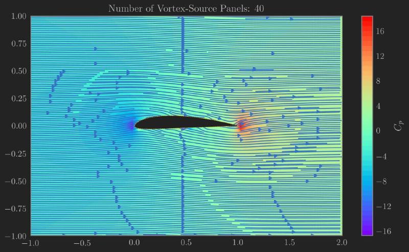
Boundary element methods express the solution of some PDE on a volume by reducing it to the specification on a surface. Panel methods in aerodynamics are special cases of such expressions, in which the governing equation is Laplace’s equation in a uniform flow in the case of a steady, inviscid, incompressible fluid.

Equivalent Inviscid Flow

Governing equation

The governing equation for this problem is Laplace’s equation in 2 dimensions: $$ \nabla^2 \phi = \nabla^2\left(\Phi + \Phi_\infty\right) = 0 $$

Note that the Laplace equation is an elliptic PDE, hence boundary conditions specified at any point in the domain affect the solution at all other points in the domain.

The “physically” motivated formulation for a closed, non-porous foil is the specification of Neumann boundary conditions, which state that the normal velocity through the foil is zero and the velocity vanishes at infinity:

$$\nabla \Phi^* \cdot \hat{\mathbf n} = \nabla (\Phi + \Phi_\infty) \cdot \hat{\mathbf n} = 0, \quad \lim_{n \to \infty} \nabla \Phi = \mathbf 0$$

This implies that the potential of the interior of the body is equal to some constant $c$:

$$ \Phi_\text{int}^* = (\Phi + \Phi_\infty) = c$$

The above condition is an alternative specification in the form of a Dirichlet boundary condition on the surface boundary $\partial S$, and turns out to be more computationally efficient as the operations are on scalars rather than vectors.

Solution

Using Green’s third identity, the solution on $\partial S$ is expressed in terms of sources $\sigma$ and doublets $\phi$ of varying strength in streamwise-normal ($\hat{\mathbf s}, \hat{\mathbf n}$) coordinates:

$$ \Phi^{*}_{\text{int}}(x,y) = \Phi_{\infty}(x,y) + \frac{1}{2\pi}\int_{\partial S} \left[\sigma \ln r - \phi \frac{\partial\ln r}{\partial n}\right]\ dS, \quad \sigma = \frac{\partial\phi}{\partial n} $$

Note: Vortices are streamwise derivatives of doublets:

$$ \vec\gamma(s) = \hat{\mathbf n} \times \hat{\mathbf s}\frac{d\phi}{ds} $$

Discretisation

Discretise the equation for a foil, in which $N$ panels are assigned to the foil, and $N_w$ panels are assigned to the wake.

Assigning each panel on the foil a constant doublet strength $\phi$, and assign all panels constant source strengths $\sigma$, giving the following:

$$ \Phi_{\infty}(x,y) + \sum_{j = 1}^N \left(\frac{\sigma}{\pi}\int_{\text{panel}}\ln r \ dS\right)_j - \sum_{j = 1}^N \left(\frac{\phi}{\pi}\int_{\text{panel}}\frac{\partial\ln r}{\partial n} \ dS\right)_j = \phi_p(x,y) $$

Let: $$ B_j \equiv \frac{1}{\pi}\int_{\text{panel}}\ln r \ dS\bigg|_j, \quad A_j \equiv -\frac{1}{\pi}\int_{\text{panel}}\frac{\partial\ln r}{\partial n} \ dS\bigg|_j$$

For foil panels, we get the following system of equations:

$$ A \phi + \vec\Phi^{*} = \vec\Phi_{\infty} - B\sigma $$

Let $\vec U_s = \{~\vec U \cdot ~\hat s_i \mid 1 \leq i \leq N + N_w ~\}$.

Kutta Condition

The Kutta condition ensures the flow leaves the trailing edge “smoothly”:

$$ \Delta \phi_W = \phi_N - \phi_1 $$

The Morino condition, which equates the potential difference at the upper and lower streamlines of the trailing edge, sometimes appears to be more accurate:

$$ \phi_1 - \phi_2 = \phi_N - \phi_{N-1} $$

Cases

Now we deal with two cases:

1. Let $\Phi_{\infty}(x,y) = \Phi^{*}_\text{int}(x,y)$. This system is directly invertible for $\phi_j$ when $\sigma_j$ is specified as $\sigma_j = \vec U_\infty \cdot \hat n_j$.

$$ \vec\phi = (-A^{-1}B)\vec\sigma \equiv P\vec\sigma$$

2. Let $\sigma_j = \Phi^{*}_\text{int} = 0$, then the system is also directly invertible for $\vec\phi$ at a lower cost:

$$ \vec\phi = A^{-1} \vec\Phi_{\infty}(x,y)$$

Real Viscous Flow

Doublet Expressions

For viscous modelling, we deal with the first case using the wall transpiration model on the EIF. First, we express the edge velocities over the panels, which are the tangential derivatives of the exterior potential, expressed as sum of the internal potential and the potential ‘jump’ across the singularity distribution: $\Phi^{*}_\text{ext} = \Phi^{*}_\text{int} - \phi$. In case 1: $\Phi^{*}_\text{int} = c \in \mathbb R$, and $\phi = \Phi_{\infty} +???$.

$$ \begin{aligned} \vec u_e = \begin{cases} \vec U_s^f - \dfrac{d\phi}{ds} & \text{Airfoil} \\ & \\ \vec U_s^w - \dfrac{d}{ds}\left(A^w \phi + B^w \sigma \right) & \text{Wake} \end{cases} \end{aligned} $$

Substituting the solution for $\phi$ from case 1, we obtain the following matrix expression:

$$ \begin{aligned} \vec u_e & = \vec U_s - \frac{d}{ds} \begin{bmatrix} P \\ \hline A^w P + B^w \end{bmatrix} \vec\sigma \end{aligned} $$

Now express the sources in terms of the mass defect $m = u_e\delta^*$:

$$ \begin{aligned} \sigma_j & = \left(\frac{dm}{ds}\right)_j \\ \vec u_e & = \vec U_s - \frac{d}{ds} \begin{bmatrix} P \\ \hline A^wP + B \end{bmatrix} \frac{d\vec m}{ds} \end{aligned} $$

This gives a differential equation for $\vec u_e$.

Difference Operators

Define the following operator $\Delta^+\colon \mathbb R^n \to \mathbb R^{n-1}, n \in \mathbb N^+$ to evaluate forward differences with matrix representation:

$$ \Delta^+ \equiv \begin{bmatrix} -1 & 1 & 0 & \ldots & 0 \\ 0 & -1 & 1 & \ldots & 0 \\ \vdots & \ddots & \ddots & \ddots & \vdots \\ 0 & \ldots & -1 & 1 & 0 \\ 0 & \ldots & 0 & -1 & 1 \end{bmatrix} $$

Difference operators can be used to generically compute $n$th order differences up to desired accuracy.

The following operator $\Delta^C\colon \mathbb R^n \to \mathbb R^n$ constructs central differences with forward and backward differencing at the endpoints:

$$ \Delta^c \equiv \begin{bmatrix} -1 & 1 & 0 & \ldots & 0 \\ -1/2 & 0 & 1/2 & \ldots & 0 \\ \vdots & \ddots & \ddots & \ddots & \vdots \\ 0 & \ldots & -1/2 & 0 & 1/2 \\ 0 & \ldots & 0 & -1 & 1 \end{bmatrix} $$

Boundary Layer Equations

The thin shear boundary layer equations are obtained via the defect formulation and the thin shear approximations of the Navier-Stokes equations.

$$ \begin{aligned} \frac{d\theta}{ds} + (H + 2 - M_e^2)\frac{1}{u_e}\frac{du_e}{ds} - \frac{c_f}{2} & = 0 \quad (\textsf{Momentum}) \\ \frac{1}{\theta^*}\frac{d\theta^*}{ds} + \left(\frac{2H^{**}}{H^*} + 3 - M_e^2\right)\frac{1}{u_e}\frac{du_e}{ds} - 2c_\mathcal{D} & = 0 \quad (\textsf{Kinetic Energy}) \end{aligned} $$

where $H\equiv \delta^*/\theta$ is the momentum shape parameter, $c_f \equiv \tau_w/\frac{1}{2}\rho_e u_e^2$ is the shear stress coefficient normalised with respect to the freestream edge velocity, $M_e \equiv u_e/a_e$ is the local Mach number at the edge, $H^* \equiv \theta^*/\theta$ is the kinetic energy shape parameter, $H^{**} \equiv \delta^{**}/\theta$ is the density shape parameter, $c_\mathcal D \equiv \mathcal D / \rho_e u_e^3$ is the power dissipation coefficient.

$\textsf{Kinetic Energy} - H^*(\textsf{Momentum})$ gives the kinetic energy shape parameter equation:

$$ \begin{aligned} \implies \theta\frac{dH^*}{ds} + \left[2H^{**} + H^*(1 - H)\right]\frac{\theta}{u_e}\frac{du_e}{ds} - 2c_\mathcal{D} + H^*\frac{c_f}{2} & = 0 \end{aligned} $$

Closure Relations

The following functional dependencies are used to close the system:

$$ \begin{aligned} H^* & = H^*(H) \\ C_f & = C_f(H, Re_\theta) \\ C_\mathcal D & = C_\mathcal D(H, Re_\theta) \end{aligned} $$

where $H_k$ is the kinematic shape parameter, derived by Whitfield as:

$$ H_k = \frac{H - 0.290M_e^2}{1 + 0.113M_e^2} $$

Laminar Closure

Falkner-Skan:

Turbulent Closure

Turbulent Magic

$$ \frac{\delta}{C_\tau} \frac{dC_\tau}{ds} = 4.2\left(\sqrt{C_{\tau_{EQ}}} - \sqrt{C_\tau}\right) $$

Discretisation

The equations are discretised using central differencing, in which the variables are defined on the panel nodes.

Note: Each singularity from the inviscid formulation is at the midpoint of each panel. The edge velocities from this computations are at the nodes, hence $N$ panels with $N+1$ edge velocities.

$$ \Delta x = \frac{x_{i+1} - x_{i-1}}{2}, ~x_a = \frac{x_{i+1} + x_{i-1}}{2} $$

Resulting in the following discrete BL equations:

$$ \begin{aligned} \frac{\Delta\theta}{\Delta s} + \left(\frac{\delta_a^*}{\theta_a} + 2 - M_e^2\right)\frac{1}{u_{e_a}}\frac{\Delta u_e}{\Delta s} - \frac{c_{f_a}}{2} & = 0 \\ \frac{\Delta H^*}{\Delta s} + H_a^*(1 - H_a)\frac{\theta_a}{u_{e_a}}\frac{\Delta u_e}{\Delta s} - 2c_{\mathcal{D}_a} + H_a^*\frac{c_{f_a}}{2} & = 0 \end{aligned} $$

Residual Equations

$$ \begin{aligned} \nabla^2 \phi & = 0, \quad \rho_e \mathbf u_e \cdot \mathbf n = \Lambda\\ \frac{d\theta}{ds} + (H + 2 - M_e^2)\frac{1}{u_e}\frac{du_e}{ds} - \frac{c_f}{2} & = 0 \\ \frac{1}{\theta^*}\frac{d\theta^*}{ds} + \left(\frac{2H^{**}}{H^*} + 3 - M_e^2\right)\frac{1}{u_e}\frac{du_e}{ds} - 2c_\mathcal{D} & = 0 \end{aligned} $$

Discretisation

The discretised inviscid and viscous equations form the following system of equations to be solved for $m,~\theta,~\tilde n$.

$$ \begin{aligned} \mathbf u_e - \mathbf U_s + \frac{d}{ds} \begin{bmatrix} P \\ \hline A^wP + B \end{bmatrix} \frac{\Delta (\mathbf u_e \boldsymbol\delta^*)}{\Delta s} & = \mathcal R_1(\mathbf m) \\ \frac{\Delta\theta}{\theta} + \left(H + 2\right)\frac{\Delta u_e}{u_{e_a}} - \frac{c_{f_a}\Delta s}{2} & = \mathcal R_2(\mathbf m, \boldsymbol \theta, \tilde{\mathbf n}) \\ \frac{\Delta H^*}{H^*_a} + \left(1 - H\right)\frac{\Delta u_e}{u_{e}} + \left(\frac{c_{f}}{2} - \frac{2C_{\mathcal D}}{H^*} \right) \frac{\Delta s}{\theta} & = \mathcal R_3(\mathbf m, \boldsymbol \theta, \tilde{\mathbf n}) \end{aligned} $$

The previous setup is sufficient for modelling flows with laminar boundary layers. The additional equations for modelling transition and turbulence are:

$$ \begin{aligned} \frac{\Delta \tilde n}{\Delta s} - \frac{d\tilde n}{dRe_\theta}(H_{a})\frac{dRe_\theta}{ds}(H_{a}, \theta_{a}) & = R_{3,i}(\mathbf m, \boldsymbol \theta, \tilde{\mathbf n}) \end{aligned} $$